Running the Relativistic Simulation
using the Two Dimensional
Motion example
This tutorial is a visual
study of two dimensional motion as observed from
different reference frames.
Please Note: Relativity is built on and modifies Newtonian
Physics. These tutorials do not attempt
to teach the user Newtonian Physics.
They assume the user already knows Newtonian Physics.
If you have not run the
simulation application before, please read the System Requirements document at
http://relativitysimulation.com/Documents/SystemRequirements.html.
If you are comfortable that
your system satisfies the requirements, or just want to try it and see what
happens, go to http://relativitysimulation.com and click the “Launch” button. The first time you run the application, it may
take a minute or two to load. When it is
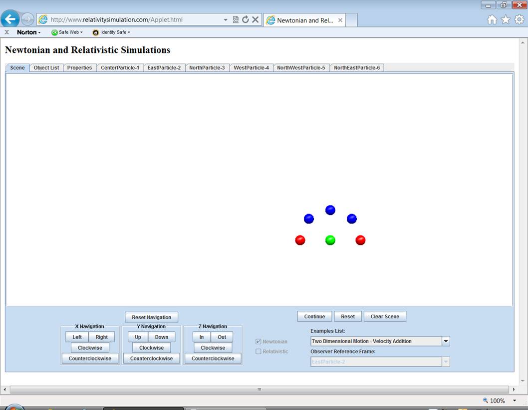
successfully loaded, you will see the blank simulation scene below.
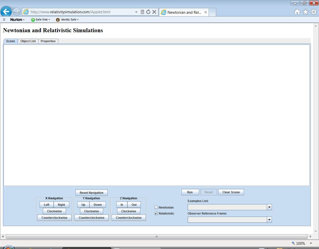
The
above picture was taken on a computer running Internet Explorer 8 on Windows
Vista. What you see on your computer may vary.
Notice the two checkboxes at the bottom center of the simulation
window. Simulations may be run using
either Newtonian or Relativistic physics.
The default is Relativistic, but in order to understand the way that
Special Relativity changes the way objects are observed in two (and three)
dimensional this tutorial will guide the user though some Newtonian simulations
too.
Selecting a Predefined Example
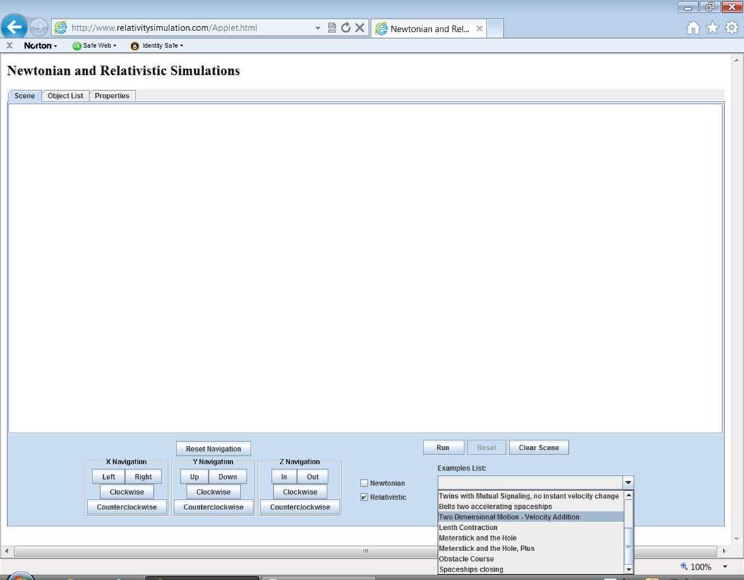
At the bottom right is a
selection box labeled Examples List.
Clicking the selection box will display a list of examples. The easiest way to use the application is to
select a predefined example from this Examples List. Your list may vary. Scroll to and select Two Dimensional
Motion – Velocity Addition.
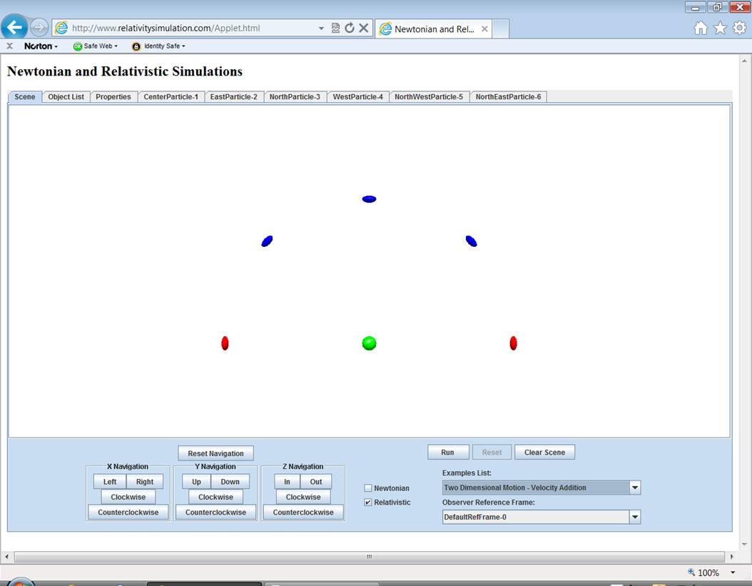
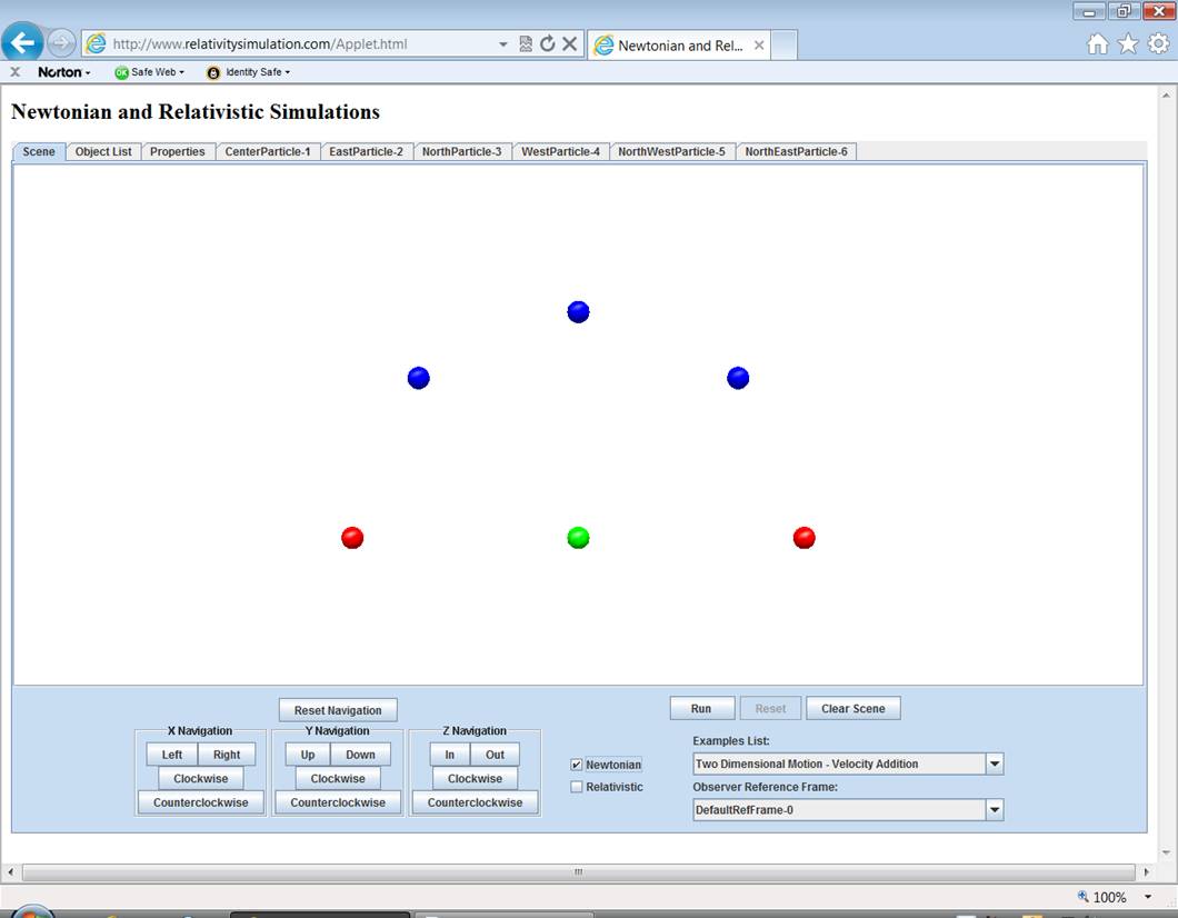
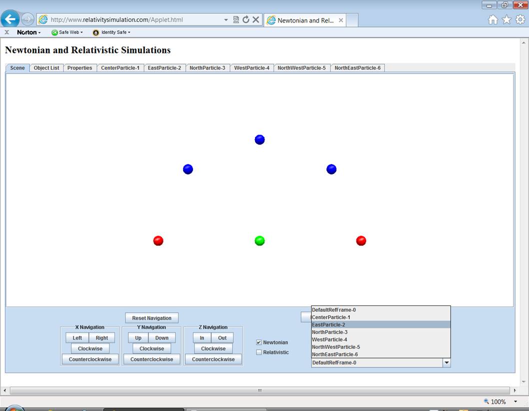
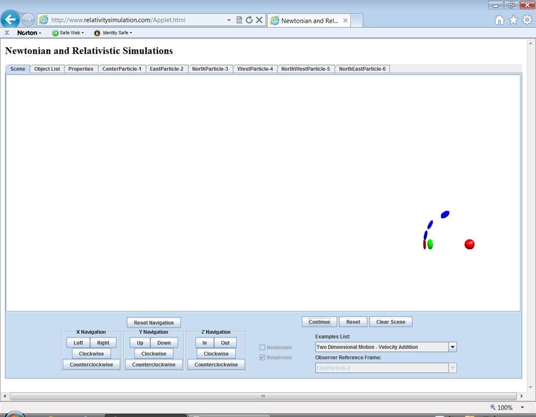
In a few seconds, you will
see three blue particles, one green and two red inserted into the scene. After the scene is populated with an example,
new tabs will appear above the scene.
The tabs will be explained in the section on Viewing and Changing
Object Properties.
Navigating through an
Example
At the bottom left of the scene
are navigation buttons. These buttons
allow you to look around the scene. The
buttons are in three groups with a reset button above. The Reset Navigation button will
cancel all navigation commands and present the scene to you as first
inserted. Buttons in the X-Navigation
group affect your view by changing your orientation with respect to the x-axis
of the scene. Similarly, there are
buttons for the y-axis and z-axis. Clicking
the Left button, for instance, will move the objects in the scene a bit
to the left. If your browser is not
showing you as much of the scene as you would like, clicking the Out
button will zoom you out a bit and show you more. To view the scene from a different angle, try
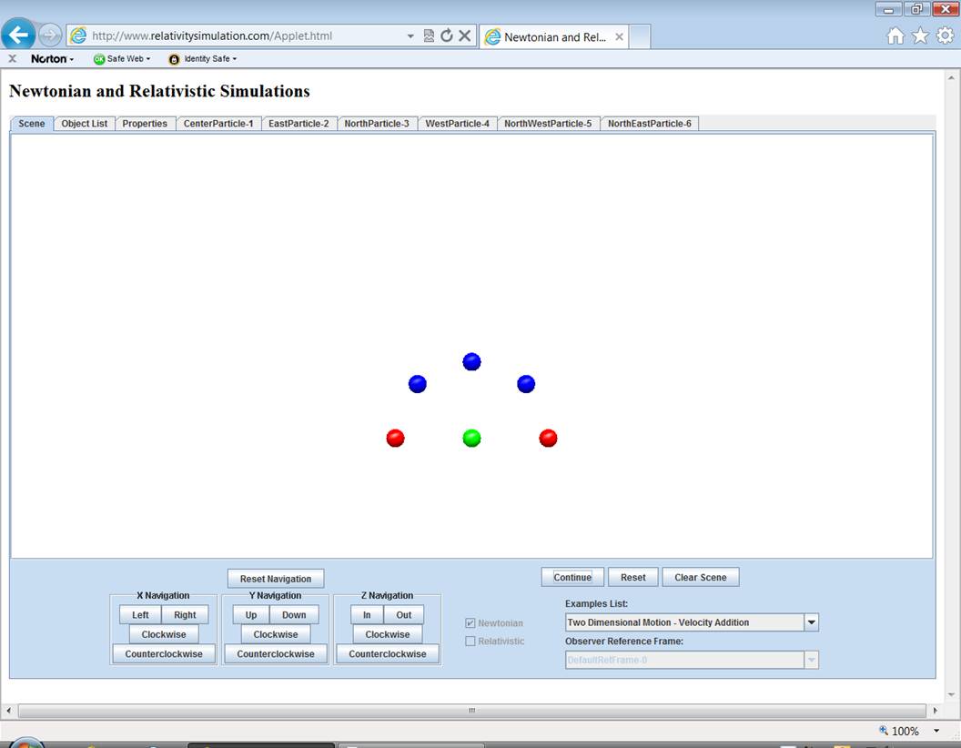
clicking a Clockwise or Counterclockwise button. If you have selected a Two Dimensional
Motion example, you are looking at a set of particles in a two dimensional
plane. The green particle and the blue
one above it are on the Y-axis. To
verify this, in the Y-axis group, click the Clockwise button a few
times.
Click Reset
Navigation. Then try clicking the Clockwise
or Counterclockwise buttons in the X-axis and Z-axis groups. Click Reset Navigation again to return
to the default view.
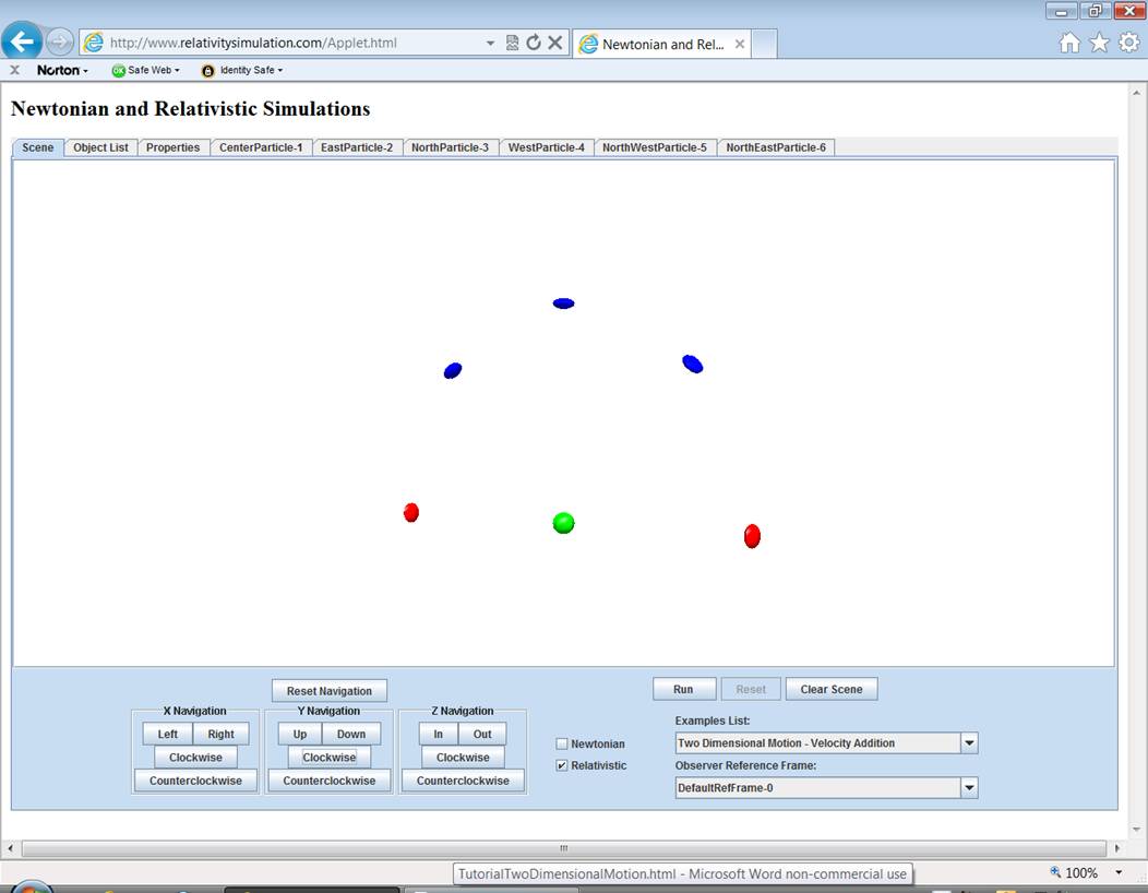
Running an Example
To run an example, at the
bottom of the scene, click the Run button. When running, the objects in the scene will
move according to the velocities and rules specified for them in their
respective properties tabs. If you have
inserted objects into the scene yourself instead of selecting an example, the
objects are initially inserted with no velocity and no rules. So clicking the run button will not do
anything. If you have selected the Two
Dimensional Motion example, clicking Run will start the three blue
and two red particles converging on the green.
Stopping an Example
If a scene is running, you
will notice that the Run button has changed its name to Stop. Click it to stop the simulation.
Continuing an Example
When stopped, the Stop
button will change its name to Continue.
Click it to continue the simulation from where it stopped.
Resetting an Example
Clicking the Reset
button will reset the objects in the scene to their initial positions ready to
run again. Click Stop and Reset now to make sure the simulation is ready for
the next section.
Switching between
Relativistic and Newtonian Simulations
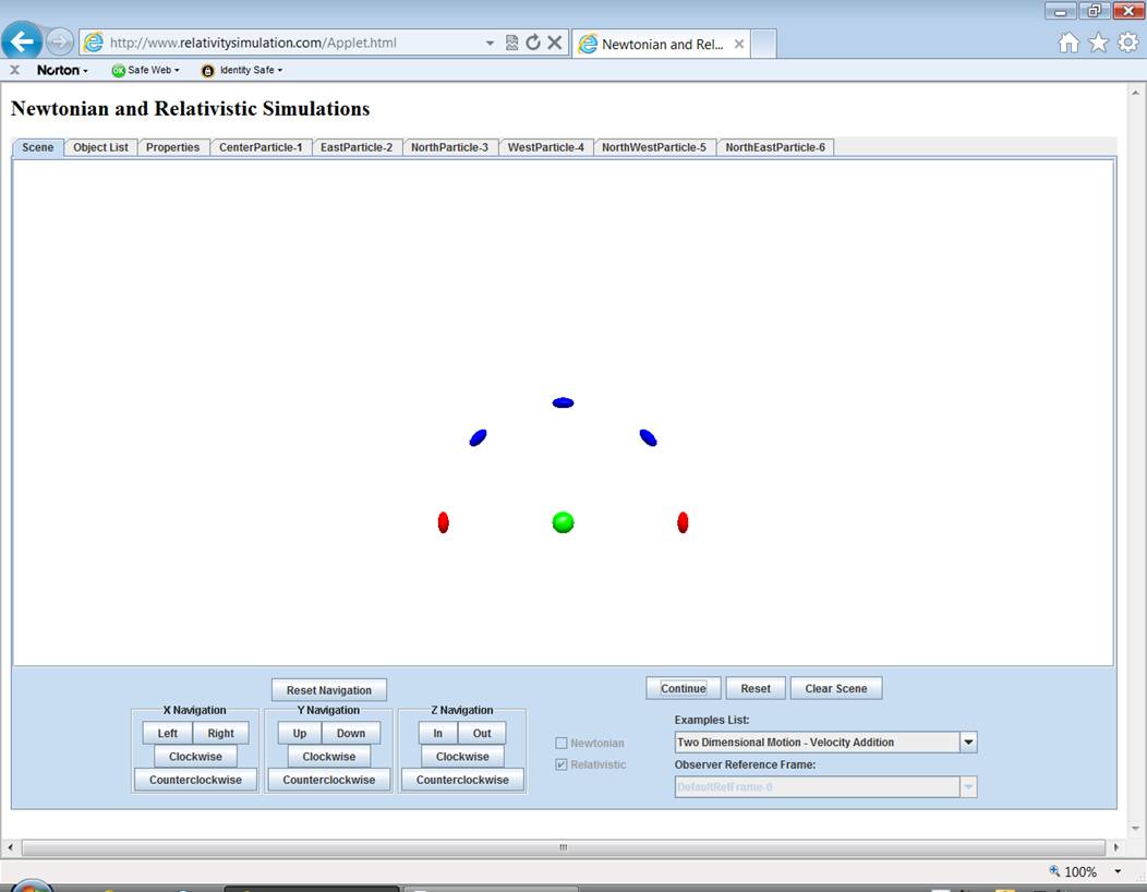
Note that the green particle
is spherical. All the other particles
are contracted by a factor of 50% in the direction of their motion. Make sure the simulation is stopped and reset
and click on the Newtonian
checkbox. This will set the simulation
to Newtonian physics where there is no contraction due to relative
velocity. Note that all the particles
are now spheres. Click Run and note that the red and blue
particles still converge on the green.
The Newtonian simulation gives the same results as the Relativistic for this reference frame.
Stop and reset the
simulation. Then run it again and make
sure to stop it before the particles converge.
Viewing and Changing
Object Properties
When an object is inserted
into the scene, it is provided with its own tab above the scene. The tabs allow you to view and change some of
the object’s properties. When you are
running a Newtonian simulation, clicking a properties tab will show you the
Newtonian properties. When running a
Relativistic simulation, clicking a properties tab will show you the
Relativistic properties for the same object.
If you have been following these instructions and have a Two
Dimensional Motion example inserted there will be one tab for each
particle. Make sure that you are running
a Newtonian simulation by verifying that the checkbox labeled Newtonian at the
bottom of the scene is checked. Then
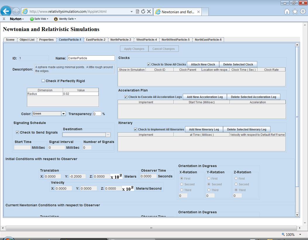
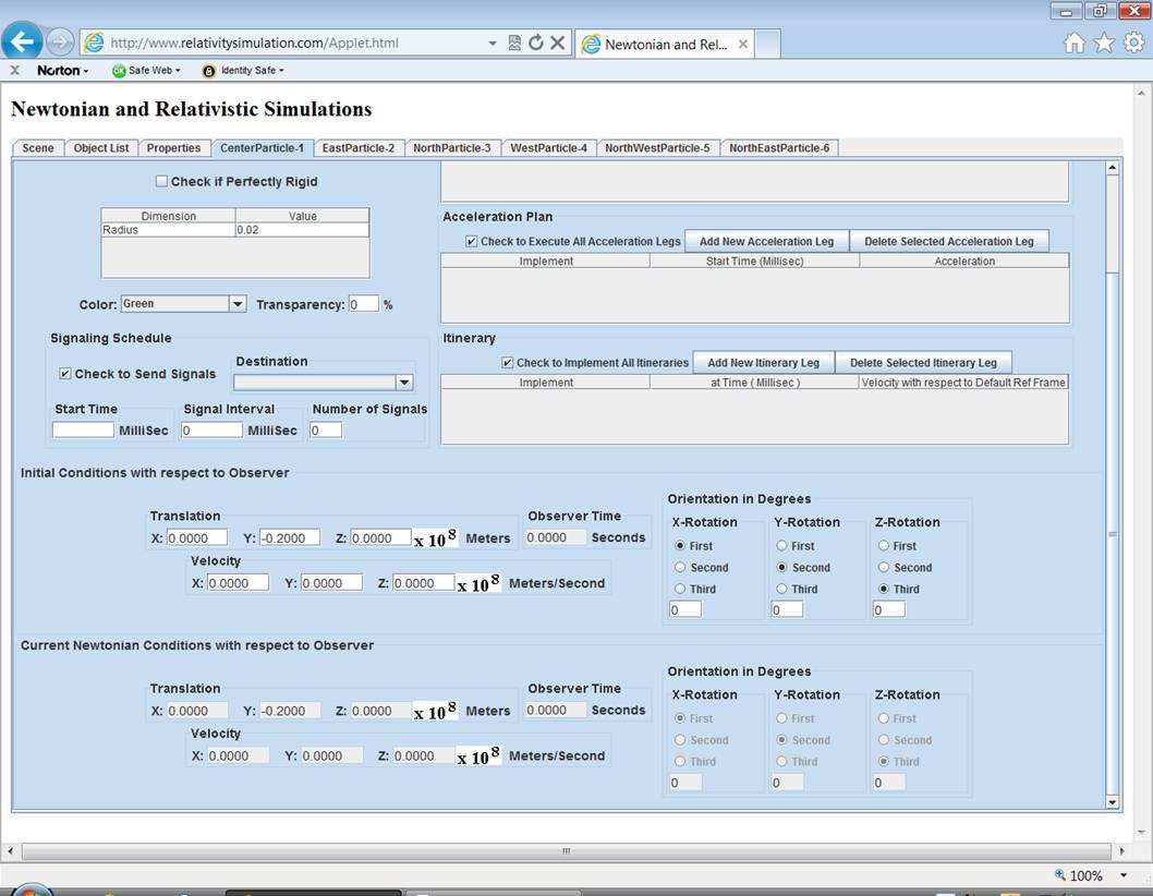
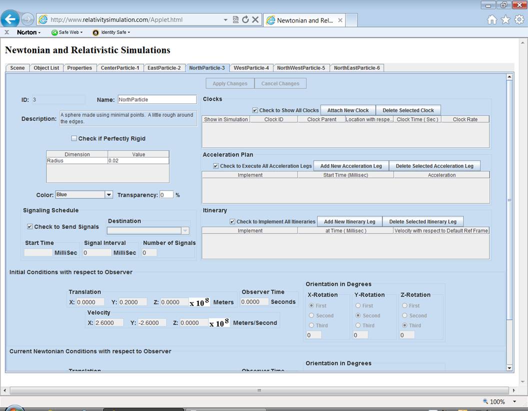
click the properties tab for CenterParticle. (The number suffix provides a unique ID when
you have more than one particle in the scene.)
You will see several sets of information. At the top left are miscellaneous properties
that may include fields for Id, name, description, rigidity, dimensions, color,
etc. Notice that the sphere’s radius is
.015. That’s 1,500,000m in this
simulation. All of the objects in all
the examples have very large sizes so as to exaggerate the time and contraction
differences predicted by Special Relativity.
To the right are sections for attached clocks, acceleration plans and
itineraries. The tutorial Pole in the Barn uses attached
clocks. The tutorial Bells Spaceships uses an acceleration
plan. Below is a section labeled Initial
Conditions with respect to Observer. The sphere’s position and velocity are
zero. Below the initial conditions is a
section entitled Current Conditions with respect to Observer.
If you don’t see it, click
the scrollbar on the right side of the window.
As long as the CenterParticle is at rest with respect to you the
observer, its current condition will be the same as its initial. Click on the tab for the EastParticle.
Note that the initial and current velocity of this particle is -260,000,000
meters/second (westerly).
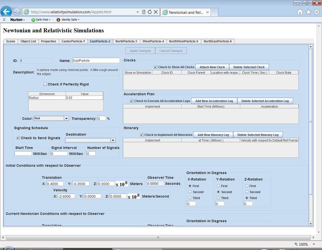
If
you have been following the tutorial and ran the simulation a little and then
stopped it, you will notice that the current translation is not the same as the
initial. It, along with the other
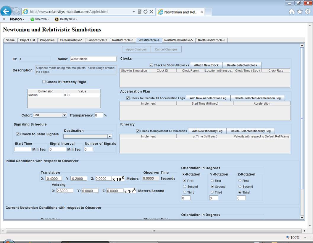
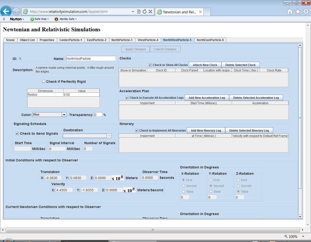
particles, is converging on the green particle. Click on the tabs for the WestParticle and examine its velocity. It is 260,000,000m/s
(easterly).
If you like, click on the
tabs for the other particles and satisfy yourself that the particles will
indeed converge as the simulation demonstrates.
Then go back to the simulation.
Switching Reference Frames
One of the objectives of this
simulation is to give you, the observer, the
opportunity to see the movement of objects from different reference
frames. You can do this whenever the
simulation is stopped and reset. Click Reset.
Just below the Examples List is another selection box labeled Observer
Reference Frame. The default
reference frame is identified there.
This is also the reference frame of the green particle. This means that the green particle is at rest
with respect to you and all the others are moving. Click the down arrow of the reference frame
selection box and notice that all the particles are listed there. Select the EastParticle.
(The number is a generic ID to help you keep track in case you have more than
one particle with the same name.)
Run the simulation and note
that the EastParticle is now at rest and the
other particles converge on it.
Click on the tabs for the
various particles and satisfy yourself that the velocities have changed in
accordance with Newtonian physics. Note
that the WestParticle velocity is 520,000,000m/s eastward. That’s greater that the speed of light. Light travels at 300,000,000 m/s. That can’t happen in Relativistic
physics. The composite speeds of the North and NorthWest particles are also
greater than the speed of light.

Switching reference frames
among moving objects will result in the objects changing velocities and
position relative to you, the observer.
In Newtonian physics, even if none of the objects have a velocity
greater than the speed of light initially, switching reference frames can
result in one or more objects having a relative velocity greater that the speed
of light. Click the simulation tab to
return to the simulation. Run and
Reset the simulation until the reasons for these greater than light
velocities are obvious. In order for WestParticle, all the way over on the left, to
participate in the convergence all the way over on the right, it must have a
very large velocity. The same argument
applies for the NorthParticle at the top of
the scene, though to a lesser extent.
Click Reset and try changing reference frames to the other
particles and running the simulation.
Physicists believe that certain events in the world must be independent
of the reference frame from which they are observed. So, even though velocities and positions are
different as determined from different reference frames, the particles always
converge together. Reset the simulation
again and switch to the default reference frame. Then click the Relativistic checkbox. Note
that the contraction of the spheres returns.
Change reference frames to the EastParticle. If you lose sight of all the particles, click
the Out button until they are all
within you view.
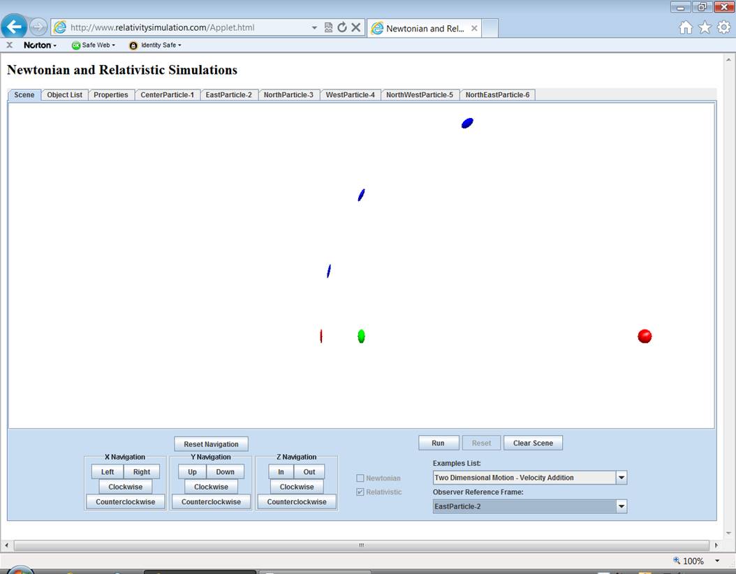
You may feel that the new
position of the particles with respect to the EastParticle is unexpected. Run the simulation, the EastParticle is at rest with respect to you and the
others move with respect to it. But all
the particles still converge. After
you’ve done this a few times you will realize the reason for the new position
of the particles. Take the WestParticle. If it had stayed in the same position
relative to the EastParticle,
it would have needed a velocity greater than the speed of light to join in the
convergence. Since it couldn’t do that
in Relativistic physics, it had to start off closer. You can check the Relativistic starting
velocities and translations of the particles by paging through the tabs.
Further experimentation:
Initial and Current Time are
included in the object properties. For
Newtonian physics, this seems a waste.
Time is absolute and every object has the same initial time and current
time. But for Relativistic physics,
every object has its own Proper Time that is a function of its position
and velocity with respect to the observer.
You, the observer, have your own time too. Reset
the simulation and review the time of the various objects in their respective
tabs. The simulation is designed to
start at observer time = zero. This is
an arbitrary choice on the part of the program.
Any object that is in the observer’s reference frame must have the
observer’s time as its Proper Time. Any
object that is not in the observer’s reference frame, but starts at the origin
of the observer’s reference frame must also have the observer’s initial time as
its Proper Time. Run the simulation
and Stop it before the convergence.
Review the time of the various objects again. Time passes for all objects but not at the
same rate. Time for you, the observer
and any object in your reference frame, passes at the fastest rate. Time for other objects passes at slower rates
depending upon the relative velocity of the object with respect to you. Click Reset. Then switch reference frames to the EastParticle.
Review the times again. Now the
EastParticle ’s initial Proper Time is zero. But CenterParticle’s
Proper Time is still zero because it is at the origin of all reference
frames.