Running the Relativistic Simulation
using the Pole in the Barn
example
This tutorial is a visual
study of the familiar Pole in the Barn Paradox. If you have not run the simulation
application before, please read the System Requirements document at http://relativitysimulation.com/Documents/SystemRequirements.html.
Please Note: Relativity is built on and modifies Newtonian
Physics. These tutorials do not attempt
to teach the user Newtonian Physics.
They assume the user already knows Newtonian Physics.
If you are comfortable that
your system satisfies the requirements, or just want to try it and see what happens,
go to http://relativitysimulation.com
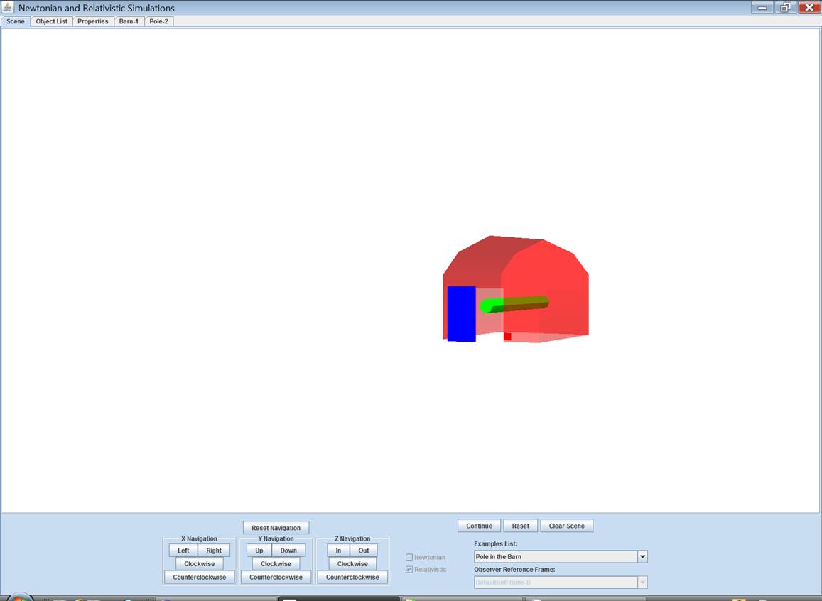
and click the “Launch” button. The first
time you run the application, it may take a minute or two to load. When it is successfully loaded, you will see
the blank simulation scene below.
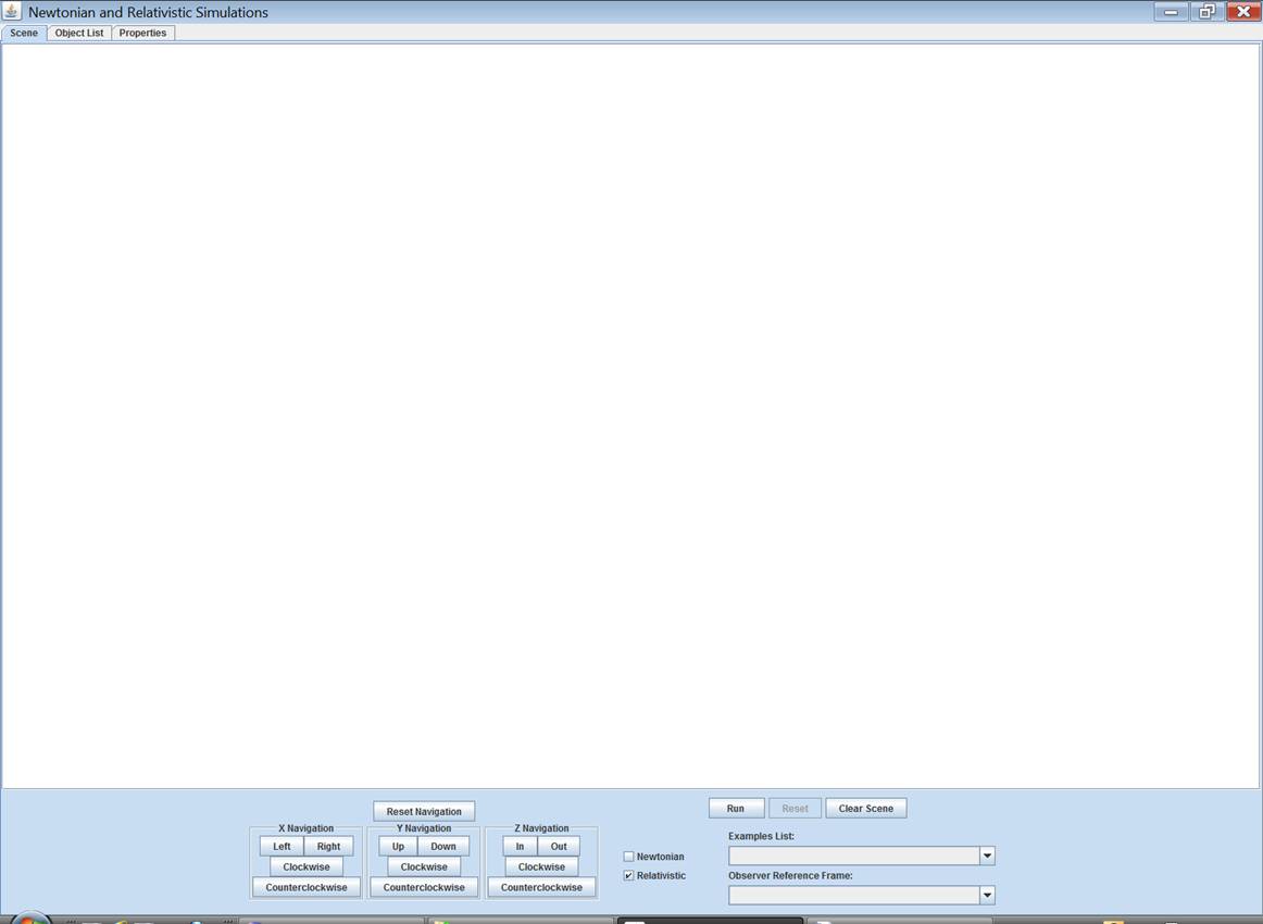
The
above picture was taken on a computer running Internet Explorer 8 on Windows
Vista. What you see on your computer may
vary. Notice the two checkboxes at the
bottom center of the simulation window.
Simulations may be run using either Newtonian or Relativistic
physics. The default is relativistic and
that is what this tutorial is for.
Selecting
a Predefined Example
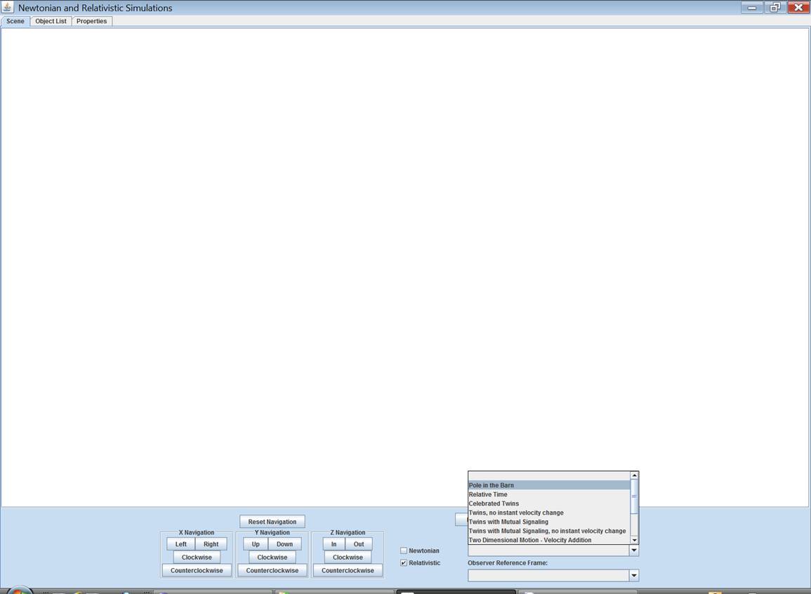
At the bottom right is a
selection box labeled Examples List.
Clicking the selection box will display a list of examples. The easiest way to use the application is to
select a predefined example from this Examples List. The list may vary. Scroll to and select Pole in the Barn.
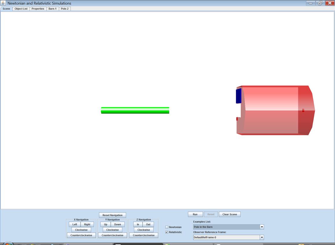
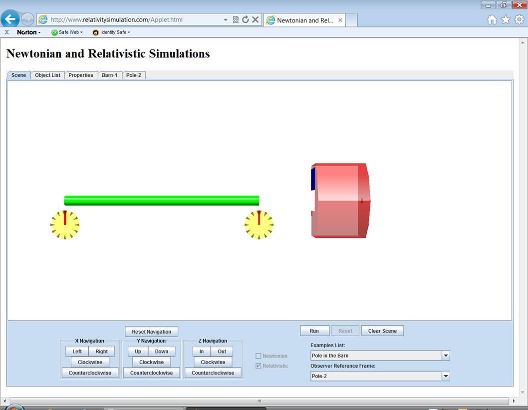
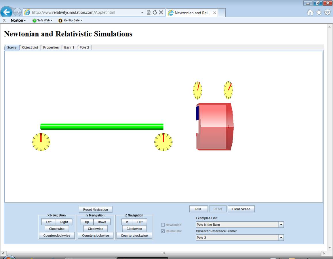
In a few seconds, you will
see a green pole and a red barn inserted into the scene. After the scene is populated with an example,
new tabs will appear above the scene.
The tabs will be explained in the section on Viewing and Changing
Object Properties.
Navigating
through an Example
At
the bottom left of the scene are navigation buttons. These buttons allow you to look around the
scene. The buttons are in three groups
with a reset button above. The Reset
Navigation button will cancel all navigation commands and present the scene
to you as first inserted. Buttons in the
X-Navigation group affect your view by changing your orientation with respect
to the x-axis of the scene. Similarly,
there are buttons for the y-axis and z-axis.
Clicking the Left button, for instance, will move the objects in
the scene a bit to the left. If your
browser is not showing you as much of the scene as you would like, clicking the
Out button will zoom you out a bit and show you more. To view the scene from a different angle, try
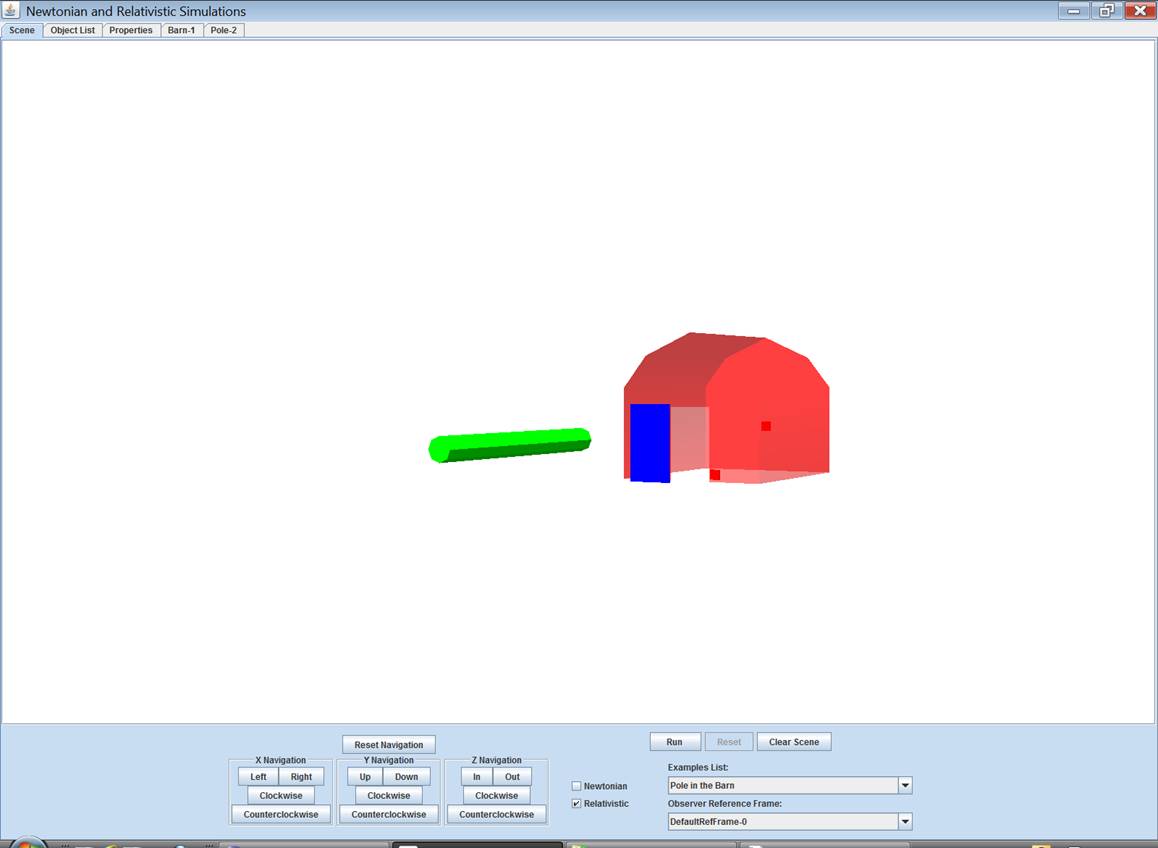
clicking a Clockwise or Counterclockwise button. If you have selected Pole in the Barn,
the example is loaded with you, the observer, looking at the barn from
above. To get a ground level view, in
the X- Navigation group, click the Clockwise button about 9 times and
then, in the Y- Navigation group, click the Counterclockwise button
about 6 times.
Running
an Example
To
run an example, at the bottom of the scene, click the Run button. When running, the objects in the scene will
move according to the velocities and rules specified for them in their
respective properties tabs. Note that if
you have inserted objects into the scene yourself instead of selecting an
example, the objects are initially inserted with no velocity and no rules. So clicking the run button will not do
anything. If you have selected the Pole
in the Barn example, clicking Run will start the pole moving toward
the barn. This example has a rule that pauses the simulation to alert the user when the pole hits
the sensor on the back wall of the barn.
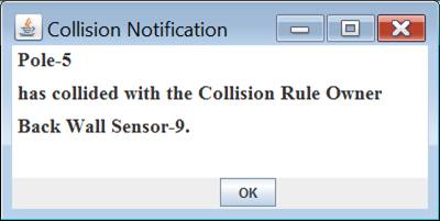
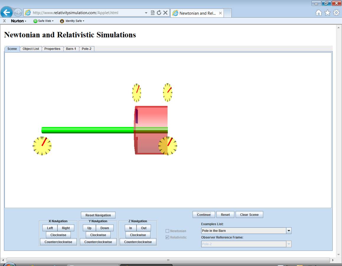
Click
OK to close the message window. Notice that the run button now says
continue. Click Continue. The pole continues
thru the back wall of the barn. At the
same time, another rule triggers the barn door to close. If the barn door encounters the pole while
closing, it will stop (jam) before it completely closes. But in this case, the door successfully
closes behind the pole.
Stopping
an Example
If
a scene is running, you will notice that the Run button has changed its
name to Stop. Click it to stop
the simulation.
Continuing
an Example
When
stopped, the Stop button will change its name to Continue. Click it to continue the simulation from
where it stopped.
Resetting
an Example
Clicking
the Reset button will reset the objects in the scene to their initial
positions ready to run again.
Switching
Reference Frames
One
of the objectives of this simulation is to give you the opportunity to observe
the movement of objects from different reference frames. You can do this whenever the simulation is
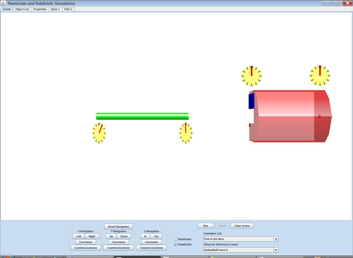
stopped and reset. If you have selected
the Pole in the Barn example, for instance, it is initially inserted
into the scene with you, the observer, in a default reference frame. This default also happens to be the reference
frame of the barn. That is, the barn is
at rest with respect to you and the pole is moving. Just below the Examples List is
another selection box labeled Observer Reference Frame. The default is identified there. Click Reset. (If Reset is not active, try clicking Stop
first.) Then Click the down arrow of the
reference frame selection box and select Pole. (The numbers after the object names are
generic IDs useful if you have more than one of the same objects in the
scene.)
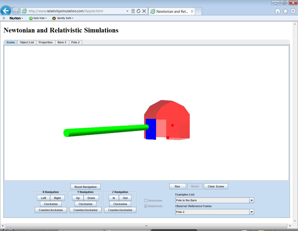
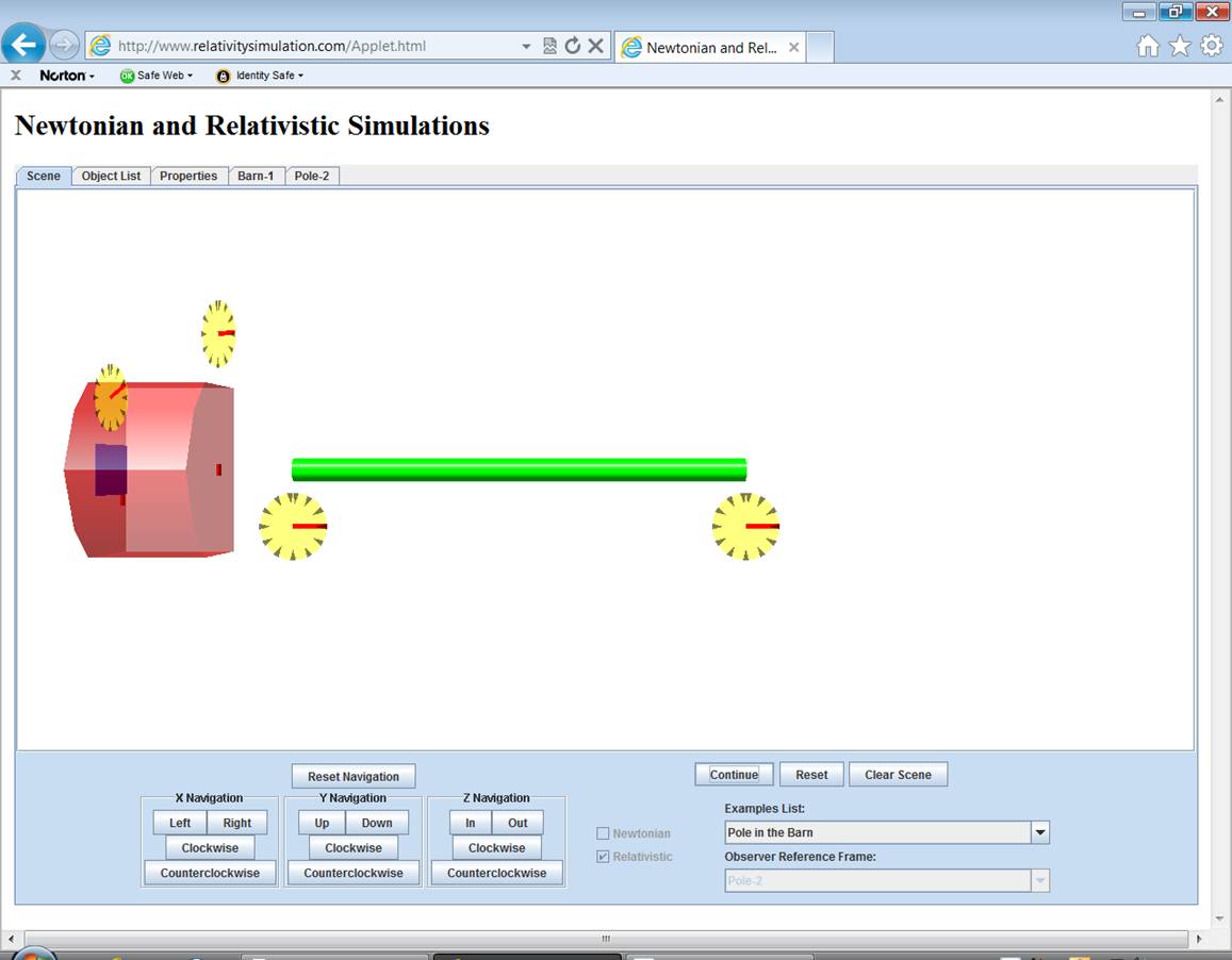
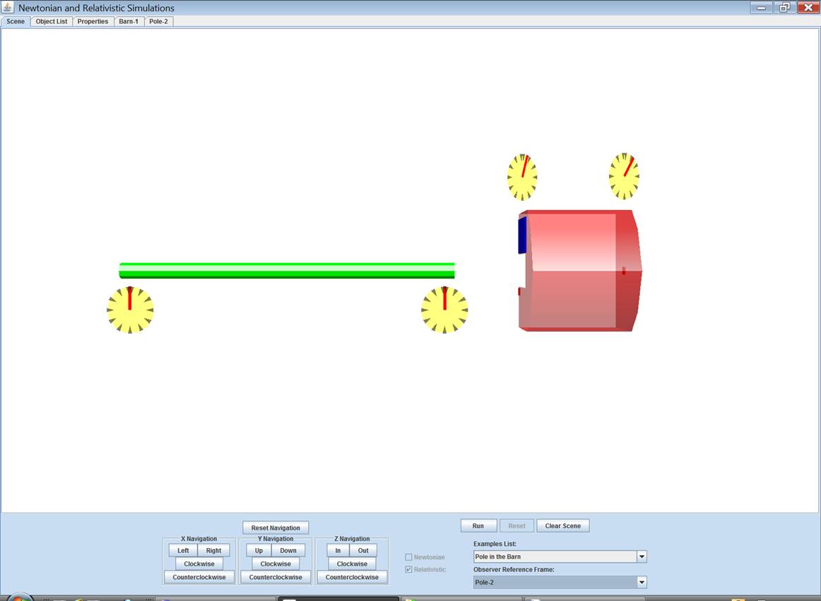
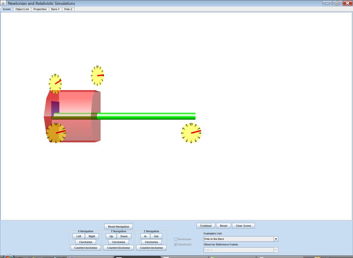
Now
it is the pole that is at rest and the barn is moving. Notice that the pole has lost is relativistic
length contraction. It is longer. The barn, on the other hand, has acquired
length contraction. It is foreshortened. Physicists believe that certain events in the
world must be independent of the reference frame from which they are
observed. So, even though velocities,
positions and geometries are different as observed from different reference
frames, if the door closed successfully in one reference frame it must do so in
all others. But how can such a long pole
get thru the short barn before the door closes?
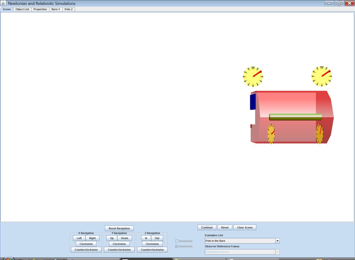
This is the reason the example is called a paradox. Run the simulation. Notice that the pole does indeed make it
thru. (You may want to use the
navigation buttons to get a better view.)
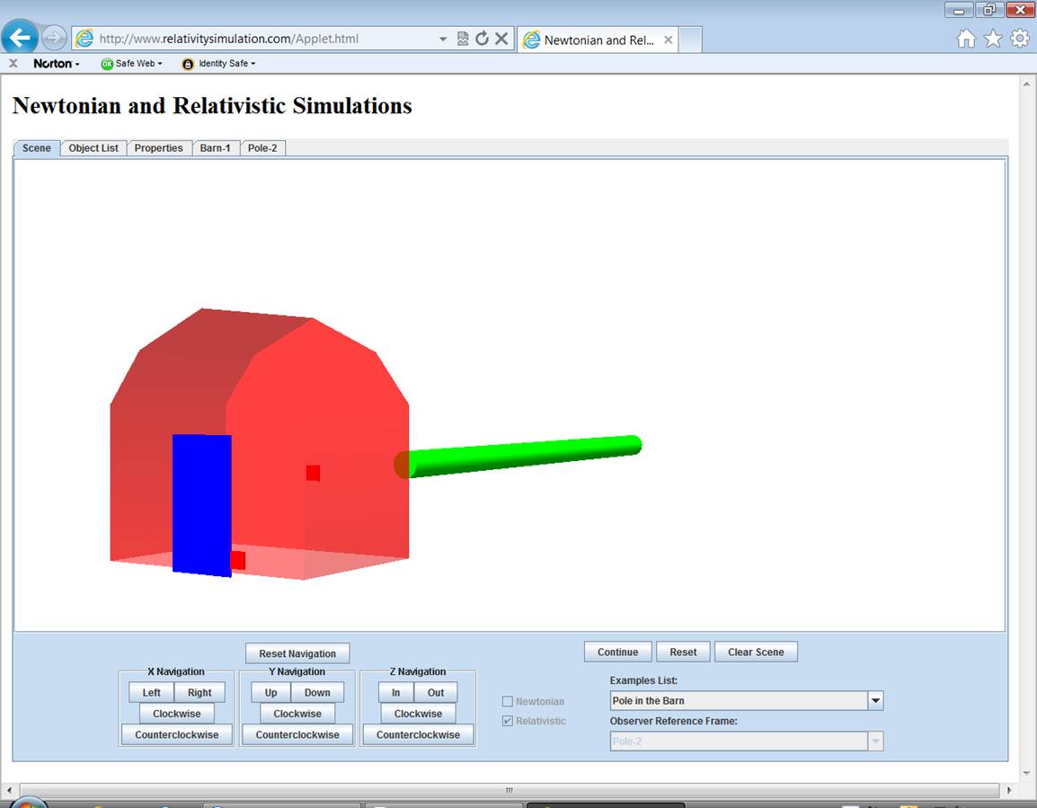
Now,
someone grounded in Newtonian physics might conclude that the program has been
“fixed”. The door no longer starts its
closure when the pole hits the back wall.
It starts much later. This is a
case of the Relativity of Simultaneity.
To better understand this characteristic of Special Relativity, this
example is provided with the ability to show clocks at strategic
locations. The next section on Viewing
and Changing Object Properties explains how to run the simulation with the
clocks showing.
Viewing
and Changing Object Properties
When
an object is inserted into the scene, it is provided with its own tab above the
scene. The tabs allow you to view and
change some of the object’s properties.
When you are running a Newtonian simulation, clicking a properties tab
will show you the Newtonian properties.
When running a Relativistic simulation, clicking a properties tab will
show you the Relativistic properties for the same object. If you have been following these instructions
and have the Pole in the Barn example inserted there will be one tab for
the barn and one for the pole. Make sure
that the Relativistic checkbox is checked and that the pole is selected
as the observer reference frame. Click Reset. Then click the properties tab for the
pole. You will see several sets of
information. At the top left are
miscellaneous properties that may include fields for the name of the object,
description, rigidity, dimensions, color, mass and charge. Just below them is an area for specifying
signaling. Signaling is covered in the
Twins tutorial. Notice that the length
of the pole is .8 long. That’s
80,000,000m in this simulation. All of
the objects in all the examples have very large sizes so as to exaggerate the
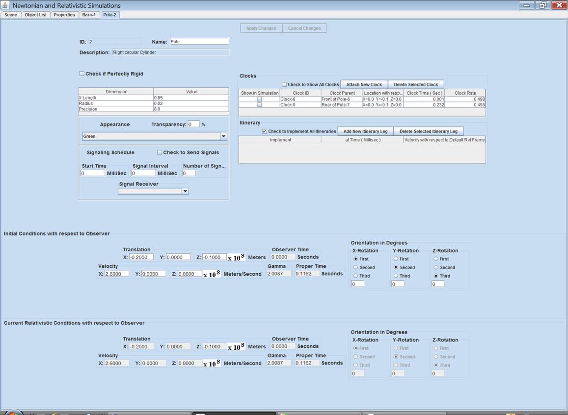
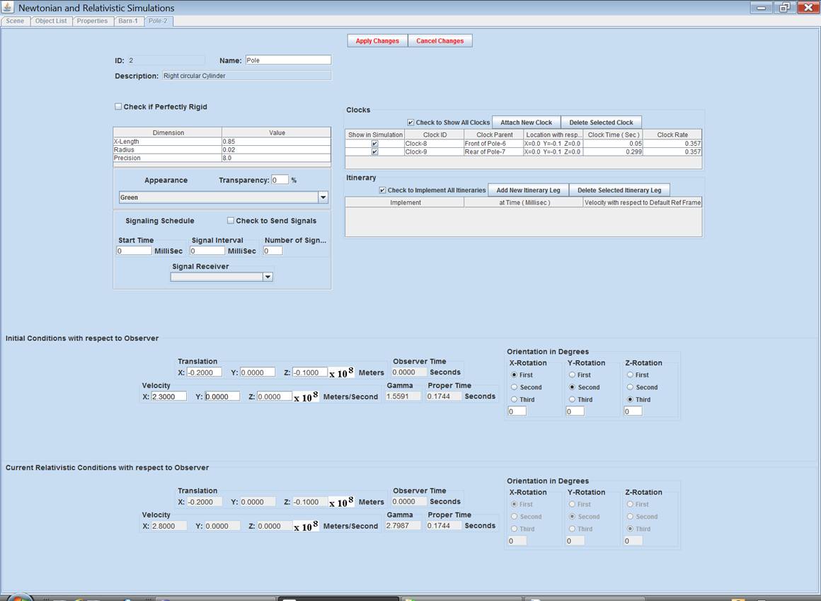
time and contraction differences predicted by Special Relativity. To the right is a section on clock
properties, acceleration plans and itineraries.
In this simulation the pole has two clocks. Below is a set of properties entitled Initial
Conditions with respect to Observer. And then a set entitled Current
Relativistic Conditions with respect to Observer. Notice that the initial translation for the
pole is x = -40,170,000m, y = 0m and z = -10,000,000m. Since the origin of the coordinate system is
the center of the scene, the scale for the scene is very large indeed! The pole’s initial velocity is zero m/s. All its rotations are 0 degrees, meaning it
is inserted into the scene with the same orientation as originally drawn. Notice that the current conditions are
identical to the initial. The pole is at
rest with respect to you. For now, just
click the checkbox Check to Show All Clocks.
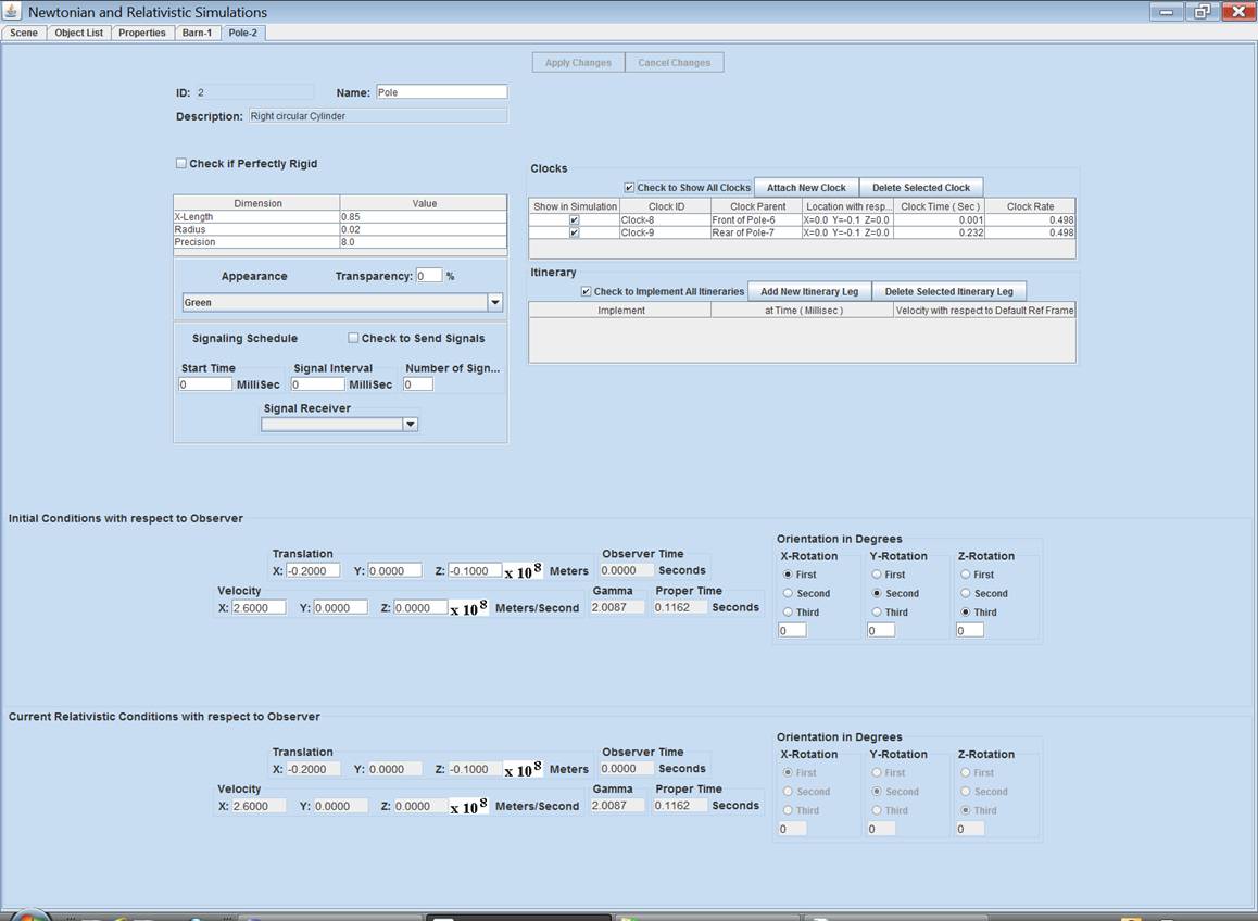
Then click the simulation
tab. If you have been doing navigation,
click the Reset Navigation button.
You will see pole and barn again plus two clocks. One will be positioned at each end of the
pole.
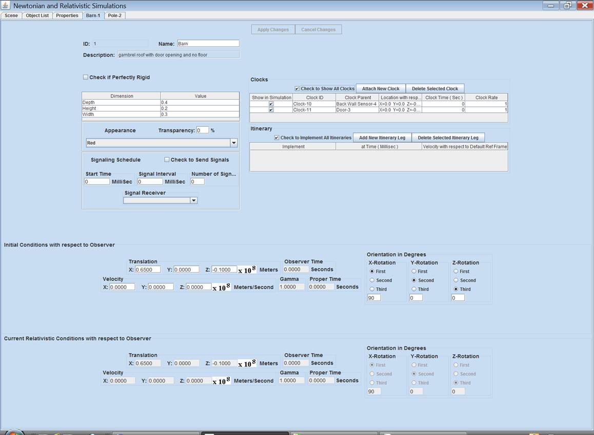
Now, click on the properties
tab for the barn. Notice that the barn
is 40,000,000m deep. Its initial
velocity is -260,000,000 meters/second in the x-direction. The barn also has two clocks. Again click the checkbox Check to Show
Clocks. Now when you go back to the
simulation, you will see two more clocks, one at the back of the barn and one
at the front.
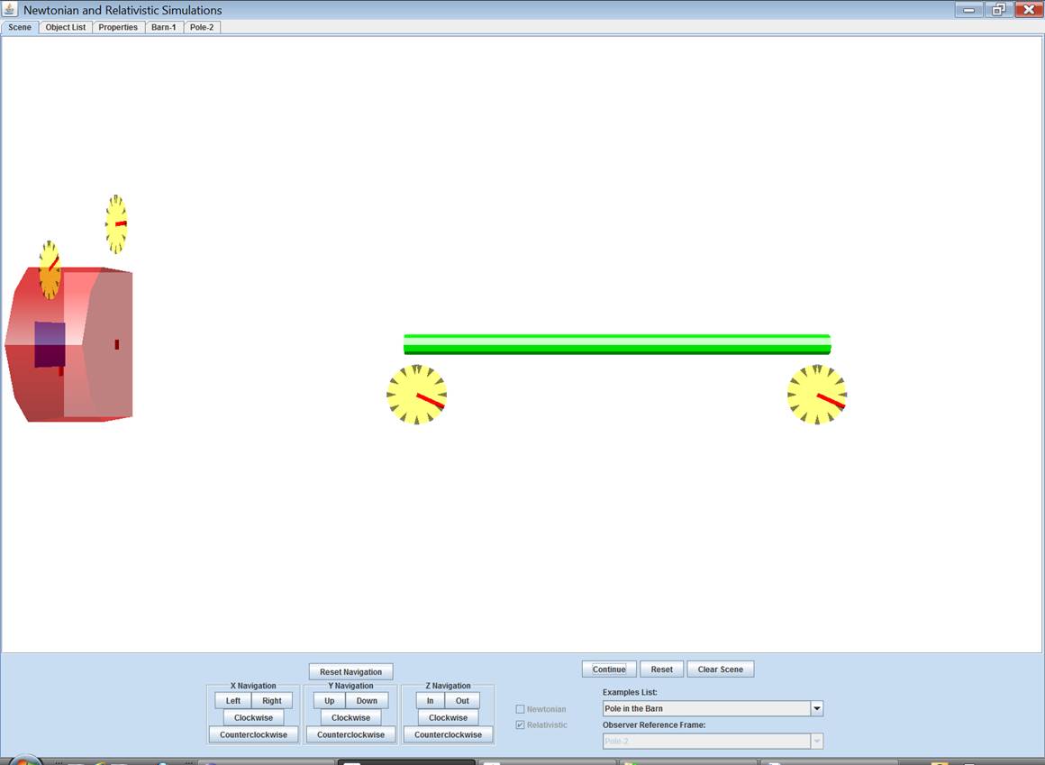
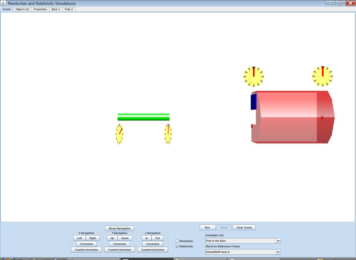
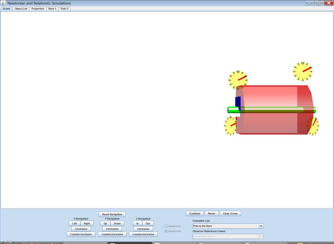
The clocks don’t have
numbers. They don’t show exact
time. They are intended to show relative
time between them. Look at the clocks on
the pole. If you have set the pole as
the observer’s reference frame, the hands on both clocks are straight up. All clocks in an observer’s reference frame
always read the same time. But the hands
on the barn clocks are not straight up and they do not agree. The time in a reference frame moving with
respect to an observer depends upon the clock’s position in and the velocity of
that reference frame. In particular,
notice that the reading on the clock at the front of the barn trails the
reading on the clock at the back. Run
the simulation until the barn hits the pole and the simulation pauses by
itself. Notice that the two clocks on
the barn have been running at half the rate of the two on the pole. Moving clocks run slow. Since the two barn clocks have been running
at the same rate, they have maintained their difference in reading with respect
to each other.
When the massage appears and
the simulation pauses, it means that the pole has hit the sensor at the back
wall of the barn and the sensor has told the barn door to close. But the sensor says close at the time as
indicated by the clock on the back wall.
That is not the time for the front of the barn and the door. The door will close when the time at the
front of the barn reads what is currently the time for the back wall. Make a note of the position of the clock hand
at the back wall then click Continue to resume the simulation. Watch the clock at the front of the barn and
notice that the door does indeed begin to close when the clock at the front of
the barn reads the noted time. The pole
has cleared the barn entrance and the door closes successfully. Length Contraction, Time Dilation and
Relativity of Simultaneity combine to produce consistent results for observers
in both reference frames.
Further experimentation
The pole and the barn are
sized such that the relative velocity of 259,600,000 meters/second between them
will demonstrate the resolution of the Pole in the Barn Paradox. This program allows you to change the size or
initial velocity of any object but you must be in the default reference frame
to do so. Click Reset and
Reset Navigation. Switch back to the
default reference frame. Then go back to
the properties tab for the pole.
Increase the velocity in the x-direction to 2.8. (Note:
When you change position or velocity parameters you must click the Apply Changes button at the top of the
page.)

Return to the simulation and
switch reference frames to the pole. Now
the barn is even more contracted. You
might instinctively think that this change will result in the door failing to
close. Try it. (You may have to click the Right button
some to see the closing.) The door
closes with room to spare.
To better understand why,
click Reset and switch back to the
default reference frame. (Click Reset Navigation too.) Now the pole is the highly contracted
object.
Run the simulation. Note how easily the highly contracted pole
clears the front of the barn before the door starts to close.
Click Reset and go to the properties tab for the Pole. Set the velocity of the pole to 2.3 in the
x-direction. Make sure to click the Apply Changes button.
Then return to the
simulation. Switch reference frames to
that of the pole. Now, with the
reference frame set as the pole, the barn is deeper.
Yet, when you run the
simulation, the door catches a piece of the pole and jams.
Click Reset and switch back to the default reference frame. Note how the not so contracted pole cannot
clear the front of the barn before the door closes.
Go back to the properties for
the pole. On the upper left side is a
dimensions table. The default length of
the pole is 80,000,000meters. Try making
the length of the pole longer or shorter and rerun the simulation. In all these cases, whether the door closes
successfully or not, the behavior observed from either the pole or the barn
should always be consistent for a given relative velocity and dimension.